Foreword
This documentation explains how to perform RFM analysis in Power BI using a dynamic, time-aware approach. In my previous documentation, I discussed a similar topic using a summary table to aggregate customer transaction data, calculate RFM scores, and assign customer segments. While that approach produced a static snapshot based on the entire dataset, this version focuses on the customer journey over time. By using a year slicer, users can select a specific year and track how customers’ purchasing behavior and RFM segments evolve across different years, rather than viewing only a single static result.
RFM Explained
RFM customer segmentation is a marketing and analytics technique that groups customers based on how recently, how frequently, and how much they purchase. It helps businesses better understand customer behavior and design more effective strategies for retention, engagement, and growth.
In this analysis, RFM is used to represent a customer’s lifetime journey rather than a static snapshot. Each component is defined as follows:
-
Recency (R): The number of days since a customer’s last purchase as of the evaluation year.
-
Frequency (F): Total number of purchases accumulated up to the evaluation year.
-
Monetary (M): Total customer spend accumulated up to the evaluation year.
Guide to IBCS Notation in this Visual (Semantic Rules)
This section explains the IBCS principles specifically implemented in this visual. The complete IBCS guidelines are available for free download on the IBCS website upon registration.
IBCS Standards 1.2 (pdf) - IBCS.com
UN 3.2 UNIFY SCENARIOS
Scenarios (also known as data categories or versions) represent different layers or assumptions within a business model. Typical scenarios include Actual, Previous Year (PY), Plan, Budget, and Forecast. Benchmarks like competitor data can also be considered scenarios. Reporting often involves showing comparisons and variances between these scenarios to provide business insights.
Three Types of Scenarios
IBCS classifies scenarios into three basic types, visually distinguished by how their visualization element (bar, column, etc.) is filled:
| Type | Description | Typical Terms |
|---|---|---|
| Actual | Data about things that have already happened. | 'Actual' (AC), 'Previous Year' (PY) |
| Planned | Data that is not yet materialized or measured. | 'Plan' (PL), 'Budget' (BU) |
| Forecasted | Data that is fictitious but incorporates measured data (e.g., a sales forecast based on measured order entry). | 'Forecast' (FC) |
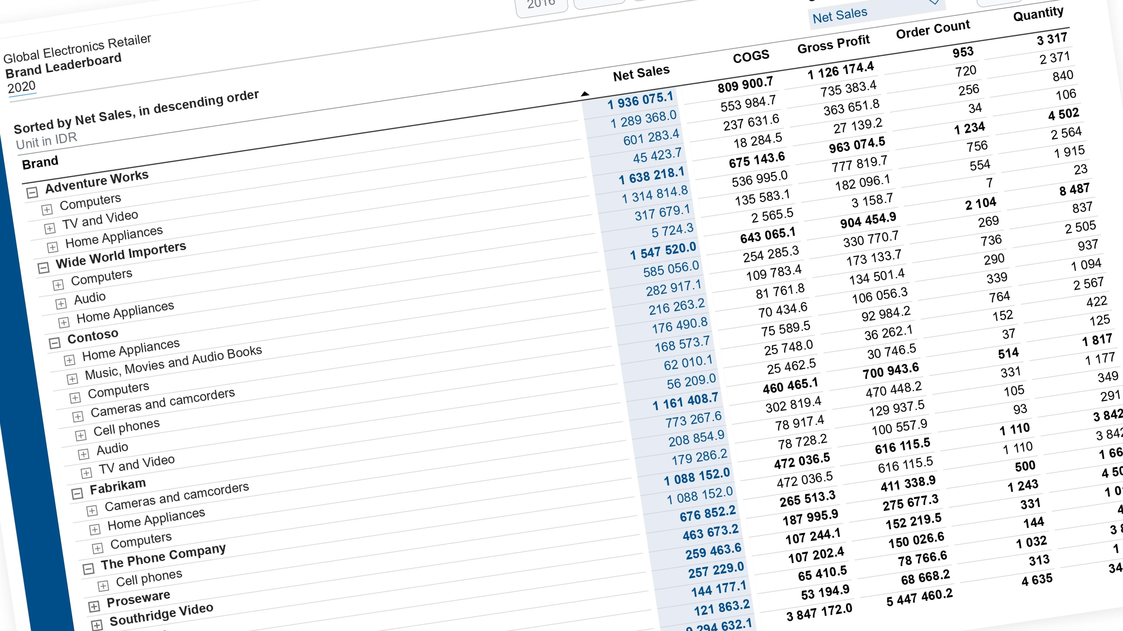
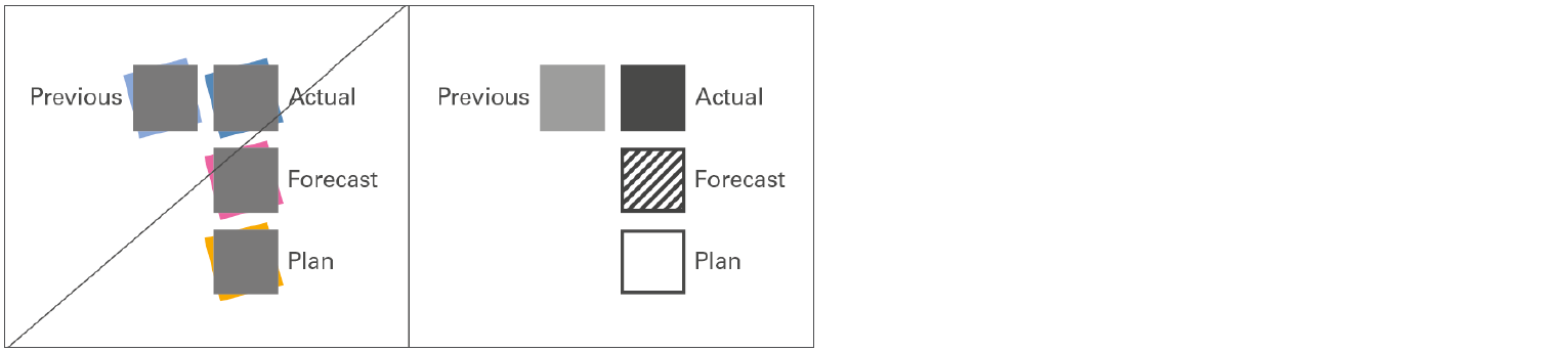 Figure UN 3.2: Unify scenarios — Source: IBCS Standards 1.2
UN 3.3: UNIFY TIME PERIODS & USE HORIZONTAL AXES
Consistent notation for time periods (for flow measures like sales) and points of time (for stock measures like inventory) is vital in all business communication. This requires standards for the visual direction of time, time abbreviations, and category widths in charts.
Visual Direction of Time Periods
Unlike structural comparisons, data series that represent change over time should always be visualized using horizontal axes.
-
In charts, time should progress from left to right.
-
In tables, time series data should also be presented in columns where time moves from left to right.
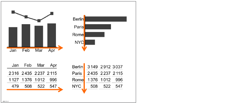 Figure UN 3.3-1: Visualization of time vs. structure (examples) — Source: IBCS Standards 1.2
Documentation
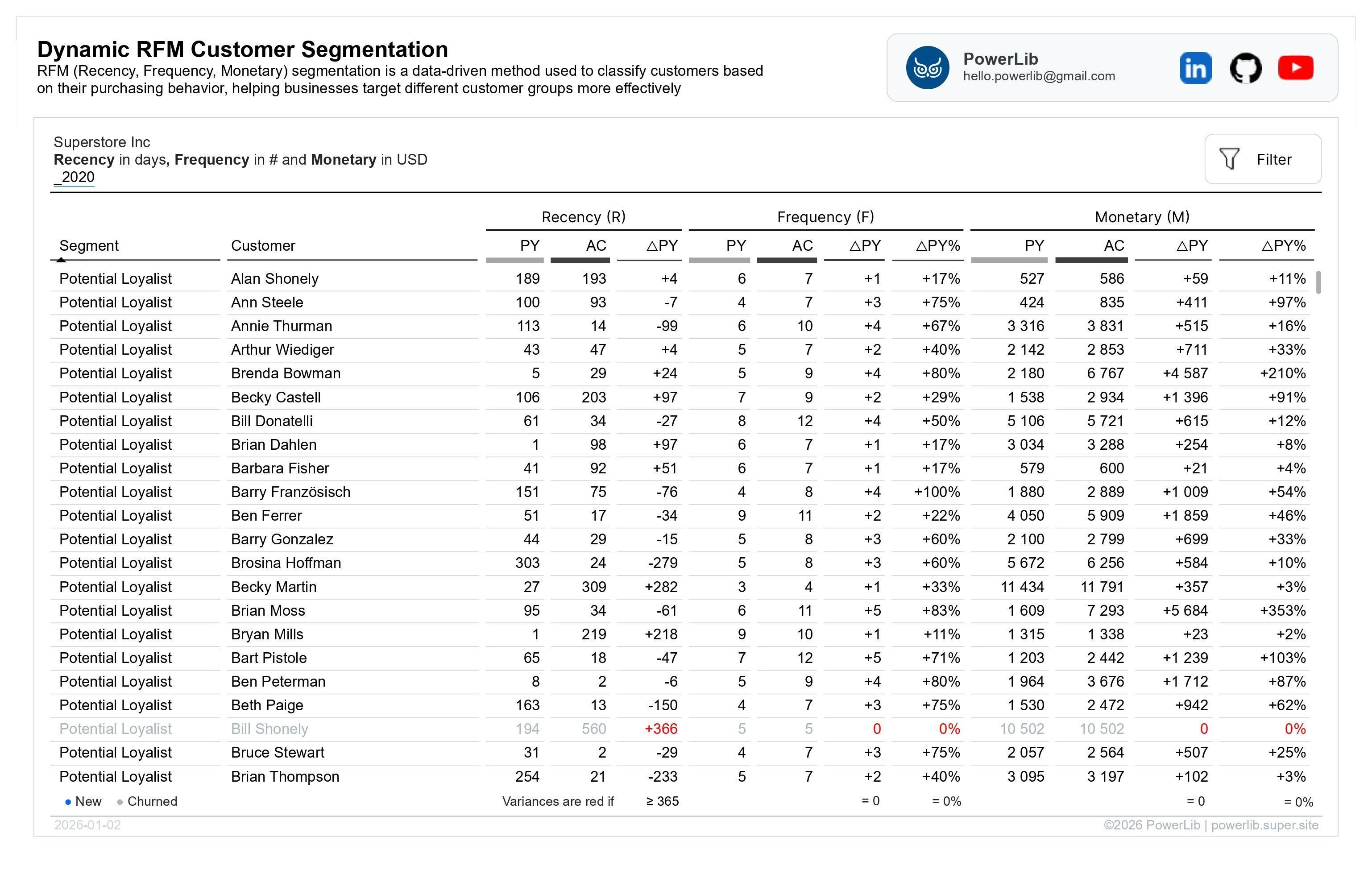 Dynamic RFM Customer Segmentation
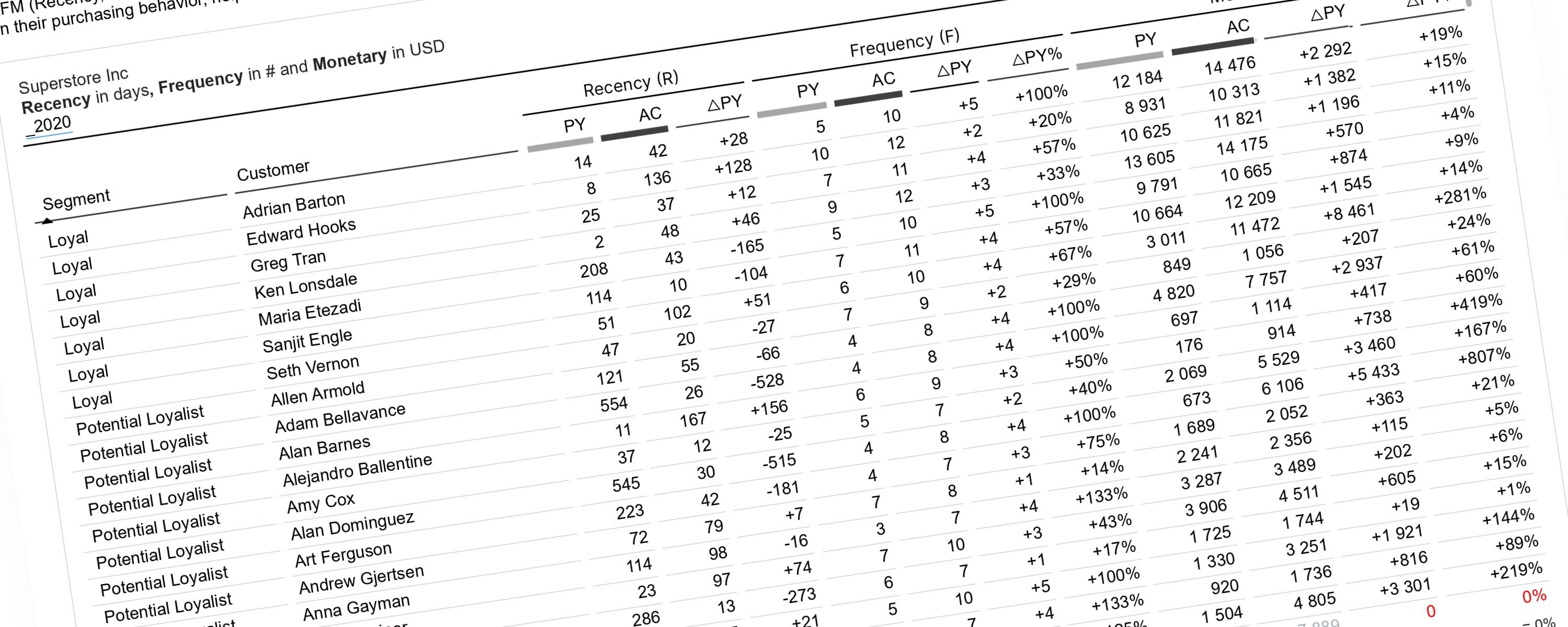
Customer Status Indicators
-
Blue-highlighted customer names represent new customers in the selected year — customers who did not make any purchases in the previous year but became active in the selected year.
-
Greyed-out customer names represent churned customers — customers who did not make any purchases in the selected year and therefore have no current-year (AC) values.
Recency (R)
Recency is displayed in days, representing the number of days between a customer’s last purchase date and the latest date within the selected year. Recency variance values of 365 days or more are highlighted in red, indicating that at least one full year has passed since the customer’s last purchase and signaling potentially churned customers.
Frequency (F)
Frequency represents the total number of transactions per customer, calculated as a running total from the earliest date in the dataset up to the selected year. This cumulative approach provides a complete view of each customer’s engagement over time. If both the absolute variance and relative variance (percentage change) are 0, it indicates that no new transactions occurred in the selected year, suggesting that the customer has churned or become inactive.
Monetary (M)
Monetary represents the total spending per customer, also calculated as a running total up to the selected year. If there is no change in total spending between the previous year and the selected year, it indicates that the customer did not make any purchases during the selected year and is therefore considered churned.
Watch the complementary video here:
Step 1: Summarizing Customer Data
To build a dynamic RFM customer segmentation, we first need to prepare the customer-level metrics required to calculate RFM scores. Instead of using a summary table, this approach relies entirely on DAX measures, allowing customer segments to update dynamically based on the selected evaluation year.
1.1 Determining the Last Order Date per Customer
To calculate Recency, we need a measure that returns the number of days between the last date of the selected year and the most recent purchase date of each customer. This calculation must be robust enough to handle different filtering scenarios driven by a year slicer.
Assume the dataset contains customer transaction data from 2017 to 2020. The measure must correctly handle the following situations:
-
Scenario 1: If a customer’s most recent purchase in the entire dataset occurs in 2020, but the user selects 2019 from the year slicer, the last order date should reflect the most recent purchase within 2019.
-
Scenario 2: If a customer’s most recent purchase occurs in 2019, and the user selects 2020 from the slicer, the last order date should still display the actual most recent purchase date (2019), even though it falls outside the selected year.
To correctly address both scenarios, we use the following DAX measure:
Measure #01: Days since last purchase per customer
_01 AC_Recency =
IF (
  NOT ISINSCOPE ( DimCustomer[Customer ID] ),
  BLANK (),
  VAR _AsOfDate =
      MAX ( DimDate[Date] )
  VAR _LastOrderDate =
      CALCULATE (
          MAX ( Superstore[Order Date] ),
          FILTER (
              ALL ( DimDate[Date] ),
              DimDate[Date] <= _AsOfDate
          )
      )
  RETURN
      DATEDIFF ( _LastOrderDate, _AsOfDate, DAY )
)

/* ============================================================================
 MEASURE: _01 AC_Recency
 PURPOSE: Calculates the number of days since a customer's last order
 CATEGORY: RFM Analysis - Recency Component
 ============================================================================

 DESCRIPTION:
 This measure calculates the "Recency" metric for RFM (Recency, Frequency,
 Monetary) analysis by determining how many days have passed since a
 customer's last order date relative to the selected date context.

 Lower recency values indicate more recent purchases (better engagement),
 while higher values indicate the customer hasn't purchased in a long time.

 ============================================================================
 BUSINESS LOGIC:
 ============================================================================
 - Recency is calculated as: Days between Last Order Date and Analysis Date
 - This is a CUMULATIVE measure - it considers all orders up to the selected date
 - Returns BLANK() for total rows to prevent meaningless aggregations
 - Only calculates at the Customer ID grain level

 ============================================================================
 TECHNICAL IMPLEMENTATION:
 ============================================================================

 STEP 1: Scope Check
 --------------------------------------------------------------------------
 IF (NOT ISINSCOPE(DimCustomer[Customer ID]), BLANK(), ...)

 - Checks if the calculation is at the customer level
 - ISINSCOPE returns TRUE when Customer ID is in the current filter context
 - Returns BLANK() for totals/subtotals to avoid incorrect aggregations
 - WHY: Recency is meaningful only at individual customer level, not aggregated

 STEP 2: Define Analysis Date
 --------------------------------------------------------------------------
 VAR _AsOfDate = MAX(DimDate[Date])

 - Captures the latest date in the current filter context
 - This becomes the "as of" date for calculating recency
 - Examples:
   * If user selects Dec 31, 2020 → _AsOfDate = 12/31/2020
   * If user selects entire 2020 → _AsOfDate = 12/31/2020
   * If no filter → _AsOfDate = last date in DimDate table

 STEP 3: Find Last Order Date (Cumulative)
 --------------------------------------------------------------------------
 VAR _LastOrderDate =
     CALCULATE(
         MAX(Superstore[Order Date]),
         FILTER(ALL(DimDate[Date]), DimDate[Date] <= _AsOfDate)
     )

 - CALCULATE: Modifies the filter context to find the last order
 - MAX(Superstore[Order Date]): Gets the most recent order date
 - FILTER(ALL(DimDate[Date]), ...): Removes existing date filters
 - DimDate[Date] <= _AsOfDate: Considers ALL orders up to the analysis date
 - WHY CUMULATIVE: This captures the customer's entire purchase history,
   not just orders within the selected period

 EXAMPLE:
 - Customer last ordered on Jan 15, 2020
 - User selects Dec 31, 2020 as analysis date
 - Even though Jan 15 is before the selection, it's still captured
 - Result: 351 days (difference between Jan 15 and Dec 31)

 STEP 4: Calculate Day Difference
 --------------------------------------------------------------------------
 RETURN DATEDIFF(_LastOrderDate, _AsOfDate, DAY)

 - DATEDIFF: Calculates difference between two dates
 - First parameter: Start date (last order date)
 - Second parameter: End date (analysis date)
 - Third parameter: Unit of measurement (DAY)
 - Result: Positive integer representing days since last purchase

 ============================================================================
 USAGE EXAMPLES:
 ============================================================================

 Example 1: Recent Customer
 - Last Order: Dec 25, 2020
 - Analysis Date: Dec 31, 2020
 - Recency: 6 days (very recent, high engagement)

 Example 2: Dormant Customer
 - Last Order: Jan 1, 2019
 - Analysis Date: Dec 31, 2020
 - Recency: 730 days (2 years inactive, at risk)

 Example 3: Visual Context
 - Matrix Visual with Customer ID in rows
 - Date slicer set to 2020
 - Each customer shows days since their last order up to Dec 31, 2020
 - Total row shows BLANK() (not applicable for aggregation)

 ============================================================================
 DEPENDENCIES:
 ============================================================================
 TABLES:
 - DimCustomer: Contains [Customer ID] dimension
 - DimDate: Contains [Date] dimension for time filtering
 - Superstore: Contains [Order Date] fact data

 RELATIONSHIPS:
 - Superstore[Order Date] → DimDate[Date] (active relationship required)
 - Superstore[Customer ID] → DimCustomer[Customer ID] (active relationship)

 DOWNSTREAM MEASURES:
 - _01 R Score: Uses this measure to assign recency scores (1-5)
 - _04 RFM Score: Combines R, F, M scores into single RFM value
 - _05 RFM Customer Segment: Assigns customers to segments based on RFM

 ============================================================================
 IMPORTANT NOTES:
 ============================================================================

 1. CUMULATIVE BEHAVIOR:
    - This measure looks at ALL historical orders, not just the selected period

 2. NULL HANDLING:
    - If customer has NO orders, _LastOrderDate will be BLANK
    - DATEDIFF with BLANK input returns BLANK (not zero)
    - These customers may need special handling in segmentation

 3. PERFORMANCE CONSIDERATIONS:
    - FILTER(ALL(DimDate[Date])) removes filters, can be expensive on large datasets
    - Consider adding KEEPFILTERS if performance issues arise
    - Works best when DimDate is properly indexed

 4. DATE CONTEXT SENSITIVITY:
    - Results change based on user's date selection
    - Always uses the MAX date in the selection as the reference point
    - Users should understand this is "recency as of [selected date]"

 5. SCORING IMPLICATIONS:
    - Lower recency = Higher R Score (5) = More valuable
    - Higher recency = Lower R Score (1) = At risk
    - Typical thresholds: 0-200 days (5), 200-400 (4), 400-600 (3), etc.

 ============================================================================
 TROUBLESHOOTING:
 ============================================================================

 Issue: All customers show same recency value
 Solution: Check if Customer ID is in the visual's row/column context

 Issue: Recency shows BLANK for all customers
 Solution: Verify Superstore[Order Date] relationship to DimDate is active

 Issue: Negative recency values
 Solution: Check data quality - Order Date should not be in the future

 Issue: Unexpected values when date slicer changes
 Solution: Expected behavior - recency is calculated "as of" selected date

 ============================================================================
 VERSION HISTORY:
 ============================================================================
 Version: 1.0
 Created: 2026-01-09
 Author: Iwa Sanjaya
 Last Modified: 2026-01-18

 Change Log:
 - 1.0: Initial creation for cumulative RFM analysis

 ============================================================================
*/
This measure calculates how many days have passed since a customer's last order (their "recency"). A lower number means the customer ordered more recently.
Read the Explanation
Step 1: Context Check
IF (
  NOT ISINSCOPE ( DimCustomer[Customer ID] ),
  BLANK (),
The measure first checks if we're looking at individual customers. If not (for example, if you're viewing a total across all customers), it returns blank because recency only makes sense at the customer level.
Step 2: Get the Reference Date
VAR _AsOfDate =
  CALCULATE (
      MAX ( DimDate[Date] ),
      ALL ( DimDate ),
      DimDate[Year] = _Year
  )
It captures the current date being analyzed from your date slicer or filter (stored as _AsOfDate). This is your "as of" date - the point in time you're measuring from.
Step 3: Find the Last Order Date
VAR _LastOrderDate =
      CALCULATE (
          MAX ( Superstore[Order Date] ),
          FILTER (
              ALL ( DimDate[Date] ),
              DimDate[Date] <= _AsOfDate
          )
      )
The measure searches through all order dates up to and including the reference date to find when this specific customer last placed an order. It ignores any date filters to ensure it sees the complete order history.
Step 4: Calculate Days Since Last Order
RETURN
      DATEDIFF ( _LastOrderDate, _AsOfDate, DAY )
)
Finally, it counts the number of days between the customer's last order and your reference date. This gives you the recency score.
Example: If today is January 15, 2026, and a customer last ordered on January 1, 2026, their recency would be 14 days.
1.2 Calculating the Total Number of Transactions per Customer
To assign the Frequency score, we need to calculate the total number of transactions made by each customer up to the selected evaluation year. This represents a cumulative count from the beginning of the dataset through the end of the selected year, rather than a count limited to a single year.
For example, assume that a customer has 7 total transactions across the entire dataset. If the user selects 2019 as the evaluation year, the Frequency value should reflect only the transactions made up to 2019, which might be 5 in this case.
To correctly handle this cumulative behavior, we use the following DAX measure:
Measure #02: Total number of purchases per customer (up to year-end)
_01 AC_Frequency =
VAR _AsOfDate =
  MAX ( DimDate[Date] )
RETURN
CALCULATE (
  DISTINCTCOUNT ( Superstore[Order ID] ),
  FILTER (
      ALL ( DimDate[Date] ),
      DimDate[Date] <= _AsOfDate
  )
)

/* ============================================================================
 MEASURE: _01 AC_Frequency
 PURPOSE: Calculates the total number of distinct orders per customer
 CATEGORY: RFM Analysis - Frequency Component
 ============================================================================

 DESCRIPTION:
 This measure calculates the "Frequency" metric for RFM (Recency, Frequency,
 Monetary) analysis by counting how many distinct orders a customer has made
 up to and including the selected date context.

 Higher frequency values indicate more loyal, repeat customers, while lower
 values indicate one-time or occasional buyers.

 ============================================================================
 BUSINESS LOGIC:
 ============================================================================
 - Frequency is calculated as: Count of Unique Orders per Customer
 - This is a CUMULATIVE measure - it considers all orders up to the selected date
 - Uses DISTINCTCOUNT to ensure each order is counted only once
 - Automatically respects customer filter context when used in visuals
 - Can aggregate to totals (unlike Recency measure)

 ============================================================================
 TECHNICAL IMPLEMENTATION:
 ============================================================================

 STEP 1: Define Analysis Date
 --------------------------------------------------------------------------
 VAR _AsOfDate = MAX(DimDate[Date])

 - Captures the latest date in the current filter context
 - This becomes the cutoff date for counting orders
 - Examples:
   * If user selects Dec 31, 2020 → _AsOfDate = 12/31/2020
   * If user selects Q1 2020 → _AsOfDate = 03/31/2020
   * If user selects Jan 15, 2020 → _AsOfDate = 01/15/2020
   * If no filter → _AsOfDate = last date in DimDate table
 - WHY MAX: Ensures we get the end of the selected period for cumulative count

 STEP 2: Count Distinct Orders (Cumulative)
 --------------------------------------------------------------------------
 RETURN CALCULATE(
     DISTINCTCOUNT(Superstore[Order ID]),
     FILTER(ALL(DimDate[Date]), DimDate[Date] <= _AsOfDate)
 )

 - CALCULATE: Modifies the filter context to count all historical orders
 - DISTINCTCOUNT(Superstore[Order ID]): Counts unique orders
   * WHY DISTINCTCOUNT: Prevents double-counting if Order ID appears multiple times
   * Each order should be counted once, regardless of line items
 - FILTER(ALL(DimDate[Date]), ...): Removes existing date filters
   * ALL(DimDate[Date]): Clears any date filters from slicers/visuals
   * Creates a blank canvas to apply custom date filter
 - DimDate[Date] <= _AsOfDate: Includes ALL orders from beginning through analysis date
 - WHY CUMULATIVE: Frequency should reflect customer's lifetime order count,
   not just orders within a selected period

 CUMULATIVE BEHAVIOR EXAMPLE:
 Customer Order History:
 - Order 1: Jan 10, 2019
 - Order 2: Jun 15, 2019
 - Order 3: Mar 20, 2020
 - Order 4: Nov 5, 2020

 Scenario A: User selects "All Time"
 Result: Frequency = 4 orders

 Scenario B: User selects "2020"
 Result: Frequency = 4 orders (still counts 2019 orders!)
 Analysis Date = Dec 31, 2020, so ALL orders up to that date count

 Scenario C: User selects "Q1 2020"
 Result: Frequency = 3 orders
 Analysis Date = Mar 31, 2020, so only orders through Q1 2020 count

 ============================================================================
 USAGE EXAMPLES:
 ============================================================================

 Example 1: High Frequency Customer (Loyal)
 - Customer has placed 25 orders since joining
 - Analysis Date: Dec 31, 2020
 - Frequency: 25 (indicates high loyalty, repeat buyer)

 Example 2: Low Frequency Customer (One-time buyer)
 - Customer has placed 1 order
 - Analysis Date: Dec 31, 2020
 - Frequency: 1 (potential target for retention campaigns)

 Example 3: New Customer
 - Customer joined Dec 2020, placed 2 orders
 - Analysis Date: Dec 31, 2020
 - Frequency: 2 (new but showing promise)

 Example 4: Matrix Visual Usage
 - Rows: DimCustomer[Customer ID], DimCustomer[Customer Name]
 - Values: [_01 AC_Frequency]
 - Date Slicer: 2020
 - Result: Each customer shows total orders from beginning through Dec 31, 2020
 - Total Row: Sum of all customer frequencies (total orders in database)

 Example 5: Time Intelligence Comparison
 - Card 1: [_01 AC_Frequency] with Year = 2020 → Total orders through 2020
 - Card 2: [_01 AC_Frequency] with Year = 2019 → Total orders through 2019
 - Difference: Shows orders placed in 2020

 ============================================================================
 DEPENDENCIES:
 ============================================================================
 TABLES:
 - DimDate: Contains [Date] dimension for time filtering
 - Superstore: Contains [Order ID] fact data
 - DimCustomer: Implicitly used through relationship context

 COLUMNS:
 - Superstore[Order ID]: Unique identifier for each order (must be distinct)
 - Superstore[Order Date]: Date when order was placed
 - DimDate[Date]: Date dimension table

 RELATIONSHIPS:
 - Superstore[Order Date] → DimDate[Date] (active relationship required)
 - Superstore[Customer ID] → DimCustomer[Customer ID] (filters frequency by customer)

 DOWNSTREAM MEASURES:
 - _02 F Score: Uses this measure to assign frequency scores (1-5)
   * Typical thresholds: 1-3 orders (1), 4-6 (2), 7-9 (3), 10-12 (4), 13+ (5)
 - _04 RFM Score: Combines R, F, M scores into single RFM value
 - _05 RFM Customer Segment: Assigns customers to segments based on RFM

 ============================================================================
 KEY DIFFERENCES FROM RECENCY:
 ============================================================================

 1. NO ISINSCOPE CHECK:
    - Unlike _01 AC_Recency, this measure doesn't check for Customer ID scope
    - WHY: Frequency can be meaningfully aggregated (total orders)
    - Works at customer level AND grand total level

 2. AGGREGATABLE:
    - Total row shows sum of all orders (meaningful business metric)
    - Recency total would be meaningless (can't average "days since last order")

 3. ALWAYS POSITIVE:
    - Frequency is always >= 0 (count of orders)
    - Recency can vary widely and requires interpretation

 4. SIMPLER LOGIC:
    - Single CALCULATE statement (no nested variables)
    - Recency requires two variables (_AsOfDate and _LastOrderDate)

 ============================================================================
 IMPORTANT NOTES:
 ============================================================================

 1. CUMULATIVE BEHAVIOR:
    - This measure looks at ALL historical orders, not just the selected period
    - "Frequency as of [selected date]" = lifetime orders up to that date
    - For period-specific analysis, use "_01 AC_Frequency (Period)" instead

 2. DISTINCTCOUNT IMPORTANCE:
    - Critical to use DISTINCTCOUNT, not COUNT or COUNTROWS
    - Superstore table may have multiple rows per Order ID (line items)
    - DISTINCTCOUNT ensures each order is counted once

    Example:
    Order ID: ORD-001
    - Line 1: Product A, $10
    - Line 2: Product B, $20
    - Line 3: Product C, $15

    COUNT would return 3 (wrong!)
    DISTINCTCOUNT returns 1 (correct - one order with three items)

 3. NULL HANDLING:
    - If customer has no orders, result is 0 (not BLANK)
    - DISTINCTCOUNT of empty set = 0
    - These customers will receive F Score of 1 (lowest)

 4. PERFORMANCE CONSIDERATIONS:
    - FILTER(ALL(DimDate[Date])) can be expensive on large date tables
    - Consider using KEEPFILTERS for better performance in some scenarios
    - Index on Superstore[Order ID] improves DISTINCTCOUNT performance
    - Relationship optimization: Ensure Order Date → Date relationship is active

 5. DATA QUALITY REQUIREMENTS:
    - Order ID must be unique per order (not per line item)
    - Order Date must be populated for all orders
    - Missing Order Dates will exclude those orders from the count

 6. SCORING IMPLICATIONS:
    - Higher frequency = Higher F Score (5) = More valuable customer
    - Lower frequency = Lower F Score (1) = One-time buyer
    - Typical thresholds (customize based on your business):
      * 1-3 orders: Score 1 (Infrequent)
      * 4-6 orders: Score 2 (Occasional)
      * 7-9 orders: Score 3 (Regular)
      * 10-12 orders: Score 4 (Frequent)
      * 13+ orders: Score 5 (Very Frequent/Loyal)

 ============================================================================
 TROUBLESHOOTING:
 ============================================================================

 Issue: Frequency values seem too high
 Solution: Check if Order ID is truly unique per order (not per line item)
          Verify with: DISTINCTCOUNT(Superstore[Order ID]) vs COUNT(Superstore[Order ID])

 Issue: Frequency shows 0 for customers with orders
 Solution: Check Superstore[Order Date] → DimDate[Date] relationship is active
          Verify Order Date values are not NULL

 Issue: Frequency doesn't change when date slicer changes
 Solution: Expected for recent dates - cumulative measure includes all history
          Only decreases when selecting earlier dates

 Issue: Total doesn't match sum of customer frequencies
 Solution: Possible duplicate Order IDs across customers (data quality issue)
          Each order should belong to only one customer

 Issue: Performance is slow with large datasets
 Solution: 1) Ensure Order ID column is indexed
          2) Consider materialized aggregation tables
          3) Check date table size (reduce if possible)

 ============================================================================
 TESTING & VALIDATION:
 ============================================================================

 Test 1: Verify Distinctness
 - Create measure: Test = COUNTROWS(Superstore) / DISTINCTCOUNT(Superstore[Order ID])
 - If result > 1, you have multiple rows per order (expected for line items)
 - If result = 1, you may have data quality issues (only one item per order?)

 Test 2: Validate Cumulative Behavior
 - Pick a customer, note their frequency on Dec 31, 2020
 - Change date to Dec 31, 2019
 - Frequency should be equal or lower (never higher)

 Test 3: Cross-Check with Source Data
 - Filter Superstore to one customer
 - Count distinct Order IDs manually
 - Compare with measure result

 Test 4: Null Date Handling
 - Identify orders with NULL Order Date
 - These should NOT be counted in frequency

 ============================================================================
 RELATED MEASURES:
 ============================================================================

 Complementary Measures:
 - _01 AC_Recency: Days since last order
 - _01 AC_Monetary: Total revenue from customer

 ============================================================================
 VERSION HISTORY:
 ============================================================================
 Version: 1.0
 Created: 2026-01-09
 Author: Iwa Sanjaya
 Last Modified: 2026-01-18

 Change Log:
 - 1.0: Initial creation for cumulative RFM analysis
 ============================================================================
*/
This measure calculates how many distinct orders a customer has placed up to a specific point in time (their "frequency"). A higher number indicates a more frequent buyer.
Read the Explanation
Step 1: Get the Reference Date
VAR _AsOfDate =
  MAX ( DimDate[Date] )
It captures the current date being analyzed from your date slicer or filter (stored as _AsOfDate). This is your "as of" date - the point in time you're measuring from.
Step 2: Count Distinct Orders Up to the Reference Date
RETURN
CALCULATE (
  DISTINCTCOUNT ( Superstore[Order ID] ),
  FILTER (
      ALL ( DimDate[Date] ),
      DimDate[Date] <= _AsOfDate
  )
)
The measure counts how many unique orders exist for the customer, but only includes orders placed on or before the reference date. It removes any existing date filters first, then applies the "less than or equal to" condition to ensure an accurate historical count.
Example: If you're analyzing data as of January 15, 2026, and a customer has placed 8 orders by that date (even if some were years ago), their frequency would be 8.
1.3 Calculating the Total Spending of Each Customer
To assign the Monetary score, we need to calculate the total spending of each customer up to the selected evaluation year. In this context, total spending is defined as the sum of sales values generated by a customer over time.
Similar to the Frequency calculation, this measure uses a cumulative approach. Instead of summing sales for a single year, it aggregates all transactions from the beginning of the dataset through the end of the selected year. This ensures that the Monetary value reflects the customer’s overall contribution up to that point in time.
For example, if a customer has generated $20,000 in total sales across all years, and the selected evaluation year is 2019, the Monetary value should include only the sales recorded up to 2019, which might be $14,500.
To handle this cumulative behavior correctly, we use the following DAX measure:
Measure #03: Total spending per customer (up to year-end)
_01 AC_Monetary =
VAR _AsOfDate =
  MAX ( DimDate[Date] )
RETURN
CALCULATE (
  SUM ( Superstore[Sales] ),
  FILTER (
      ALL ( DimDate[Date] ),
      DimDate[Date] <= _AsOfDate
  )
)

/* ============================================================================
 MEASURE: _01 AC_Monetary
 PURPOSE: Calculates the total revenue generated by each customer
 CATEGORY: RFM Analysis - Monetary Component
 ============================================================================

 DESCRIPTION:
 This measure calculates the "Monetary" metric for RFM (Recency, Frequency,
 Monetary) analysis by summing all sales revenue from a customer up to and
 including the selected date context.

 Higher monetary values indicate high-value customers who contribute more
 revenue, while lower values indicate low-spending customers.

 ============================================================================
 BUSINESS LOGIC:
 ============================================================================
 - Monetary is calculated as: Total Sales Revenue per Customer
 - This is a CUMULATIVE measure - it considers all sales up to the selected date
 - Represents Customer Lifetime Value (LTV) as of the analysis date
 - Uses SUM to aggregate all sales transactions
 - Automatically respects customer filter context when used in visuals
 - Can aggregate to totals (total revenue across all customers)

 ============================================================================
 TECHNICAL IMPLEMENTATION:
 ============================================================================

 STEP 1: Define Analysis Date
 --------------------------------------------------------------------------
 VAR _AsOfDate = MAX(DimDate[Date])

 - Captures the latest date in the current filter context
 - This becomes the cutoff date for summing sales
 - Examples:
   * If user selects Dec 31, 2020 → _AsOfDate = 12/31/2020
   * If user selects Q4 2020 → _AsOfDate = 12/31/2020
   * If user selects "2020" → _AsOfDate = 12/31/2020
   * If no filter → _AsOfDate = last date in DimDate table
 - WHY MAX: Ensures we get the end of the selected period for cumulative sum

 STEP 2: Sum Sales Revenue (Cumulative)
 --------------------------------------------------------------------------
 RETURN CALCULATE(
     SUM(Superstore[Sales]),
     FILTER(ALL(DimDate[Date]), DimDate[Date] <= _AsOfDate)
 )

 - CALCULATE: Modifies the filter context to sum all historical sales
 - SUM(Superstore[Sales]): Aggregates all sales values
   * WHY SUM: Natural aggregation for monetary values
   * Includes all line items and transactions
   * Currency values should already be in base currency unit
 - FILTER(ALL(DimDate[Date]), ...): Removes existing date filters
   * ALL(DimDate[Date]): Clears any date filters from slicers/visuals
   * Creates a blank canvas to apply custom date filter
 - DimDate[Date] <= _AsOfDate: Includes ALL sales from beginning through analysis date
 - WHY CUMULATIVE: Monetary should reflect customer's lifetime spending,
   not just sales within a selected period

 CUMULATIVE BEHAVIOR EXAMPLE:
 Customer Purchase History:
 - Jan 10, 2019: $500
 - Jun 15, 2019: $1,200
 - Mar 20, 2020: $800
 - Nov 5, 2020: $2,500

 Scenario A: User selects "All Time"
 Result: Monetary = $5,000 (total lifetime value)

 Scenario B: User selects "2020"
 Result: Monetary = $5,000 (still includes 2019 purchases!)
 Analysis Date = Dec 31, 2020, so ALL sales up to that date count

 Scenario C: User selects "Q1 2020"
 Result: Monetary = $2,500 ($500 + $1,200 + $800)
 Analysis Date = Mar 31, 2020, so only sales through Q1 2020 count

 Scenario D: User selects "Nov 2020"
 Result: Monetary = $5,000 (entire lifetime through Nov 30, 2020)

 ============================================================================
 USAGE EXAMPLES:
 ============================================================================

 Example 1: High-Value Customer (VIP)
 - Customer has spent $50,000 since joining
 - Analysis Date: Dec 31, 2020
 - Monetary: $50,000 (high-value, potential Champion segment)

 Example 2: Low-Value Customer
 - Customer has spent $250 total
 - Analysis Date: Dec 31, 2020
 - Monetary: $250 (low spender, may need attention)

 Example 3: Growing Customer
 - Started with small purchases, gradually increasing
 - Total spend: $5,000
 - Analysis Date: Dec 31, 2020
 - Monetary: $5,000 (potential for upselling)

 Example 4: Matrix Visual Usage
 - Rows: DimCustomer[Customer ID], DimCustomer[Customer Name]
 - Values: [_01 AC_Monetary]
 - Date Slicer: 2020
 - Result: Each customer shows cumulative revenue from beginning through Dec 31, 2020
 - Total Row: Sum of all customer monetary values (total company revenue)

 Example 5: Combined RFM Analysis
 - Customer A: High Monetary ($20K), High Frequency (30 orders), Low Recency (5 days)
   → Champion segment
 - Customer B: High Monetary ($18K), Low Frequency (2 orders), High Recency (400 days)
   → "Cannot Lose Them but Losing" segment

 Example 6: Time Intelligence Comparison
 - Card 1: [_01 AC_Monetary] with Year = 2020 → LTV through 2020
 - Card 2: [_01 AC_Monetary] with Year = 2019 → LTV through 2019
 - Difference: Revenue generated in 2020

 ============================================================================
 DEPENDENCIES:
 ============================================================================
 TABLES:
 - DimDate: Contains [Date] dimension for time filtering
 - Superstore: Contains [Sales] fact data
 - DimCustomer: Implicitly used through relationship context

 COLUMNS:
 - Superstore[Sales]: Revenue amount per transaction/line item
 - Superstore[Order Date]: Date when order was placed
 - DimDate[Date]: Date dimension table

 RELATIONSHIPS:
 - Superstore[Order Date] → DimDate[Date] (active relationship required)
 - Superstore[Customer ID] → DimCustomer[Customer ID] (filters revenue by customer)

 DOWNSTREAM MEASURES:
 - _03 M Score: Uses this measure to assign monetary scores (1-5)
   * Typical thresholds: $0-5K (1), $5K-10K (2), $10K-15K (3), $15K-20K (4), $20K+ (5)
 - _04 RFM Score: Combines R, F, M scores into single RFM value
 - _05 RFM Customer Segment: Assigns customers to segments based on RFM

 ============================================================================
 KEY CHARACTERISTICS:
 ============================================================================

 1. NO ISINSCOPE CHECK:
    - Like _01 AC_Frequency, this measure doesn't check for Customer ID scope
    - WHY: Monetary values can be meaningfully aggregated (total revenue)
    - Works at customer level AND grand total level

 2. AGGREGATABLE:
    - Total row shows sum of all revenue (meaningful business metric)
    - Unlike Recency which returns BLANK() for totals

 3. CONTINUOUS VALUES:
    - Monetary can be any positive decimal value
    - Unlike Frequency (integer counts) or Recency (day counts)
    - Requires different binning strategy for scoring

 4. CURRENCY CONSIDERATIONS:
    - Assumes all values are in same currency
    - No currency conversion logic included
    - Format as currency in visual properties

 ============================================================================
 IMPORTANT NOTES:
 ============================================================================

 1. CUMULATIVE BEHAVIOR:
    - This measure represents Customer Lifetime Value (LTV) as of selected date
    - "Monetary as of [selected date]" = lifetime spending up to that date
    - Not just sales within the selected period

 2. RELATIONSHIP TO CUSTOMER VALUE:
    - High Monetary + High Frequency = Loyal high-value customer (Champions)
    - High Monetary + Low Frequency = Big-ticket buyer (Cannot Lose Them)
    - Low Monetary + High Frequency = Frequent small buyer (Promising)
    - Low Monetary + Low Frequency = Low-value customer (At Risk/Lost)

 3. NULL HANDLING:
    - If customer has no sales, result is BLANK (not 0)
    - SUM of empty set = BLANK
    - These customers will receive M Score of 1 or may be excluded

 4. NEGATIVE VALUES:
    - Returns can create negative sales values
    - Consider whether to include/exclude returns in your model
    - May need separate measure for Net Sales (Sales - Returns)

 5. DATA QUALITY REQUIREMENTS:
    - Sales column must be numeric (decimal/currency type)
    - Order Date must be populated for all transactions
    - Missing Order Dates will exclude those sales from calculation
    - Verify no duplicate transactions inflating totals

 6. PERFORMANCE CONSIDERATIONS:
    - FILTER(ALL(DimDate[Date])) can be expensive on large date tables
    - SUM is generally fast, but large fact tables may require optimization
    - Consider partitioning Superstore table by date
    - Columnstore index on Sales column improves performance

 7. SCORING IMPLICATIONS:
    - Higher monetary = Higher M Score (5) = More valuable customer
    - Lower monetary = Lower M Score (1) = Low-value customer
    - Typical thresholds (customize based on your business):
      * $0-5,000: Score 1 (Low Value)
      * $5,001-10,000: Score 2 (Below Average)
      * $10,001-15,000: Score 3 (Average)
      * $15,001-20,000: Score 4 (Above Average)
      * $20,001+: Score 5 (High Value/VIP)

 8. BUSINESS CONTEXT MATTERS:
    - B2C retail: Lower thresholds ($100, $500, $1,000)
    - B2B enterprise: Higher thresholds ($10K, $50K, $100K)
    - Subscription business: Annual recurring revenue
    - E-commerce: Lifetime order value

 ============================================================================
 COMPARISON WITH OTHER RFM COMPONENTS:
 ============================================================================

 RECENCY (Days):
 - Temporal measure - how recent
 - Lower is better (more recent = more engaged)
 - Cannot be aggregated meaningfully

 FREQUENCY (Count):
 - Behavioral measure - how often
 - Higher is better (more orders = more loyal)
 - Can be aggregated (total orders)
 - Integer values only

 MONETARY (Currency):
 - Financial measure - how much
 - Higher is better (more spend = more valuable)
 - Can be aggregated (total revenue)
 - Continuous decimal values
 - Most directly tied to business value

 ============================================================================
 TROUBLESHOOTING:
 ============================================================================

 Issue: Monetary values seem too high
 Solution: Check for duplicate transactions in Superstore table
          Verify each transaction is recorded once
          Check if returns are being subtracted properly

 Issue: Monetary shows BLANK for customers with orders
 Solution: Check Superstore[Order Date] → DimDate[Date] relationship is active
          Verify Sales column is not NULL
          Ensure Sales column is numeric data type

 Issue: Monetary doesn't change when date slicer changes
 Solution: Expected for recent dates - cumulative measure includes all history
          Only decreases when selecting earlier dates
          Test by selecting a date before customer's first purchase

 Issue: Negative monetary values
 Solution: Returns/refunds may be creating negative values
          Decide if returns should be included in monetary calculation
          Consider: SUM(Superstore[Sales]) - SUM(Superstore[Returns])

 Issue: Currency formatting not displaying
 Solution: Set format in Measure properties to Currency
          Verify locale settings match your currency

 Issue: Performance is slow with large datasets
 Solution: 1) Ensure Sales column is indexed
          2) Consider aggregated fact tables
          3) Partition by date if using large datasets
          4) Use DirectQuery optimization if needed

 ============================================================================
 TESTING & VALIDATION:
 ============================================================================

 Test 1: Verify Total Alignment
 - Compare [_01 AC_Monetary] total with SUM(Superstore[Sales])
 - Should be equal when no filters applied
 - Difference indicates data quality or relationship issues

 Test 2: Validate Cumulative Behavior
 - Pick a customer, note their monetary value on Dec 31, 2020
 - Change date to Dec 31, 2019
 - Monetary should be equal or lower (never higher)

 Test 3: Cross-Check with Source Data
 - Filter Superstore to one customer
 - Sum Sales manually
 - Compare with measure result

 Test 4: Customer-Level Validation
 - Create table: Customer ID | Frequency | Monetary | Average Order Value
 - Calculate: AOV = Monetary / Frequency
 - AOV should be reasonable for your business (e.g., $50-$500)

 Test 5: Null Sales Handling
 - Identify orders with NULL Sales values
 - These should NOT be counted in monetary total
 - May indicate data quality issues

 Test 6: Date Boundary Testing
 - Select specific date (e.g., Jun 30, 2020)
 - Verify monetary includes orders through Jun 30
 - Verify monetary excludes orders after Jun 30

 ============================================================================
 ADVANCED USAGE SCENARIOS:
 ============================================================================

 Scenario 1: Customer Segmentation by Value Tiers
 - Create bins: <$1K, $1K-5K, $5K-10K, $10K+
 - Use SWITCH measure to categorize customers
 - Combine with Frequency for 2D segmentation matrix

 Scenario 2: Year-over-Year LTV Growth
 - Monetary 2020: [_01 AC_Monetary] with Year = 2020
 - Monetary 2019: [_01 AC_Monetary] with Year = 2019
 - LTV Growth = Monetary 2020 - Monetary 2019
 - Shows incremental value added in 2020

 Scenario 3: Revenue Concentration Analysis
 - Top 20% customers by monetary value
 - Calculate % of total revenue from top customers
 - Pareto principle: 80/20 rule validation

 Scenario 4: Cohort Analysis
 - Group customers by first purchase date
 - Track monetary value progression over time
 - Identify best-performing acquisition cohorts

 ============================================================================
 RELATED MEASURES:
 ============================================================================

 Complementary Measures:
 - _01 AC_Recency: Days since last order
 - _01 AC_Frequency: Count of orders

 Derived Measures:
 - Average Order Value = [_01 AC_Monetary] / [_01 AC_Frequency]
 - Revenue per Customer = [_01 AC_Monetary] / DISTINCTCOUNT(DimCustomer[Customer ID])
 - Customer Lifetime Value (explicit) = [_01 AC_Monetary]

 Comparative Measures:
 - Net Revenue = [_01 AC_Monetary] - [Total Returns]
 - Gross Margin = [_01 AC_Monetary] * [Average Margin %]

 ============================================================================
 VERSION HISTORY:
 ============================================================================
 Version: 1.0
 Created: 2026-01-09
 Author: Iwa Sanjaya
 Last Modified: 2026-01-18

 Change Log:
 - 1.0: Initial creation for cumulative RFM analysis

 ============================================================================
*/
This measure calculates the total sales revenue generated by a customer up to a specific point in time (their "monetary value"). A higher number indicates a more valuable customer in terms of revenue.
Read the Explanation
Step 1: Get the Reference Date
VAR _AsOfDate =
  MAX ( DimDate[Date] )
It captures the current date being analyzed from your date slicer or filter (stored as _AsOfDate). This is your "as of" date - the point in time you're measuring from.
Step 2: Sum All Sales Up to the Reference Date
RETURN
CALCULATE (
  SUM ( Superstore[Sales] ),
  FILTER (
      ALL ( DimDate[Date] ),
      DimDate[Date] <= _AsOfDate
  )
)
The measure adds up all sales revenue for the customer, but only includes transactions that occurred on or before the reference date. It removes any existing date filters first, then applies the "less than or equal to" condition to ensure an accurate historical total.
Example: If you're analyzing data as of January 15, 2026, and a customer has spent $5,240 in total across all their orders by that date, their monetary value would be $5,240.
Step 2: Calculating the RFM Scores
Once the required customer-level metrics are in place, the next step is to assign scores for Recency, Frequency, and Monetary. Each metric is converted into a standardized score, making it easier to compare customers with different purchasing behaviors.
After scoring each dimension individually, the three scores are combined to form an RFM profile, which is then used to group customers into meaningful segments.
While there are many RFM segmentation models available, each with its own scoring rules and thresholds, this case study follows the framework provided by Bloomreach. That said, RFM scoring is highly flexible, and you are encouraged to adapt the thresholds and segment definitions to better align with your specific business context and customer behavior.
2.1 Assigning R Score
Measure #04: R Score
_01 R Score =
SWITCH(
  TRUE(),
  [AC_Recency] <= 200, 5,
  [AC_Recency] <= 400, 4,
  [AC_Recency] <= 600, 3,
  [AC_Recency] <= 800, 2,
  [AC_Recency] > 800, 1
)
This measure converts Recency (the number of days since the last purchase) into a score from 1 to 5, where more recent customers receive higher scores. In short, fewer days since the last purchase result in a higher Recency score, while a longer gap leads to a lower score.
Read the Explanation
1. How the logic works
SWITCH(
  TRUE(),
This pattern works like a top-down IF…ELSE ladder. Each condition is checked from top to bottom and the first match wins
2. Recency thresholds explained
[AC_Recency] <= 200, 5,
    [AC_Recency] <= 200, 5,
    [AC_Recency] <= 400, 4,
    [AC_Recency] <= 600, 3,
    [AC_Recency] <= 800, 2,
    [AC_Recency] > 800, 1
)
-
Customer purchased within the last 200 days is considered very recent so it gets best score (5)
-
Purchased 201–400 days ago is considered still active so it gets score 4
-
Purchased 401–600 days ago is considered average recency so it gets score 3
-
Purchased 601–800 days ago is considered becoming inactive so it gets score 2
-
Purchased more than 800 days ago so it considered very inactive so it gets lowest score (1)
2.2 Assigning F Score
Measure #05: F Score
_02 F Score =
SWITCH(
  TRUE(),
  [AC_Frequency] <= 3, 1,
  [AC_Frequency] <= 6, 2,
  [AC_Frequency] <= 9, 3,
  [AC_Frequency] <= 12, 4,
  [AC_Frequency] > 12, 5
)
This measure converts the number of purchases a customer has made into a score from 1 to 5, where more frequent buyers receive higher scores. In other words, the greater the number of purchases, the higher the Frequency score.
Read the Explanation
1. How the logic works
SWITCH(
  TRUE(),
This pattern works like a top-down IF…ELSE ladder. Each condition is checked from top to bottom and the first match wins
2. Frequency thresholds explained
[AC_Frequency] <= 3, 1,
    [AC_Frequency] <= 6, 2,
    [AC_Frequency] <= 9, 3,
    [AC_Frequency] <= 12, 4,
    [AC_Frequency] > 12, 5
)
-
Customers who made 1–3 purchases are considered very infrequent and receive a score of 1.
-
Those with 4–6 purchases are considered low frequency and receive a score of 2.
-
Customers with 7–9 purchases are considered medium frequency and receive a score of 3.
-
Those with 10–12 purchases are considered high frequency and receive a score of 4.
-
Customers with more than 12 purchases are considered very frequent and receive the highest score of 5.
2.3 Assigning M Score
Measure #06: M Score
_03 M Score =
SWITCH(
  TRUE(),
  [AC_Monetary] <= 5000, 1,
  [AC_Monetary] <= 10000, 2,
  [AC_Monetary] <= 15000, 3,
  [AC_Monetary] <= 20000, 4,
  [AC_Monetary] > 20000, 5
)
This measure converts a customer’s total spending into a score from 1 to 5, where customers who spend more receive higher scores.
Read the Explanation
i. How the logic works
SWITCH(
  TRUE(),
This pattern works like a top-down IF…ELSE ladder. Each condition is checked from top to bottom and the first match wins
ii. Monetary thresholds explained
[AC_Monetary] <= 5000, 1,
    [AC_Monetary]  <= 10000, 2,
    [AC_Monetary]  <= 15000, 3,
    [AC_Monetary]  <= 20000, 4,
    [AC_Monetary]  > 20000, 5
)
-
Customers who spent ≤ $5,000 are considered low value and receive a score of 1.
-
Those who spent $5,001–$10,000 are considered below average and receive a score of 2.
-
Customers who spent $10,001–$15,000 are considered medium value and receive a score of 3.
-
Those who spent $15,001–$20,000 are considered high value and receive a score of 4.
-
Customers who spent more than $20,000 are considered very high value and receive the highest score of 5.
2.4 Combining RFM Score
Measure #07: RFM Score
_04 RFM Score =
CONCATENATE(
  CONCATENATE( [R Score], [F Score] ),
  [M Score]
)
This measure combines the Recency, Frequency, and Monetary scores into a single 3-digit customer code.
Read the Explanation
1. Combine R and F
CONCATENATE( [R Score], [F Score] )Example: if R = 5 and F = 4, the result will be "54" (text)
2. Append M
CONCATENATE( "54", [M Score] )If M = 3, the final result will be "543"
Step 3: Segmenting Customers Based on RFM Score
Once the RFM scores are calculated, the next step is to assign customers to segments based on their combined scores. This segmentation follows the Bloomreach framework, as introduced earlier.
Measure #08: RFM Customer Segment
_05 RFM Customer Segment =
IF(
  ISINSCOPE( DimCustomer[Customer ID] ),
  VAR RFM = [RFM Score]
  RETURN
  SWITCH(
      TRUE(),
      RFM IN { "555", "554", "544", "545", "454", "455", "445" }, "Champions",
      RFM IN { "543", "444", "435", "355", "354", "345", "344", "335" }, "Loyal",
      RFM IN { "553", "551", "552", "541", "542", "533", "532", "531", "452", "451", "442", "441", "431", "453", "433", "432", "423", "353", "352", "351", "342", "341", "333", "323" }, "Potential Loyalist",
      RFM IN { "512", "511", "422", "421", "412", "411", "311" }, "New Customers",
      RFM IN { "525", "524", "523", "522", "521", "515", "514", "513", "425", "424", "413", "414", "415", "315", "314", "313" }, "Promising",
      RFM IN { "535", "534", "443", "434", "343", "334", "325", "324" }, "Need Attention",
      RFM IN { "331", "321", "312", "221", "213", "231", "241", "251" }, "About to Sleep",
      RFM IN { "155", "154", "144", "214", "215", "115", "114", "113" }, "Cannot Lose Them but Losing",
      RFM IN { "255", "254", "245", "244", "253", "252", "243", "242", "235", "234", "225", "224", "153", "152", "145", "143", "142", "135", "134", "133", "125", "124" }, "At Risk",
      RFM IN { "332", "322", "233", "232", "223", "222", "132", "123", "122", "212", "211" }, "Hibernating Customers",
      RFM IN { "111", "112", "121", "131", "141", "151" }, "Lost Customers",
      "Other"
  ),
  BLANK() // Returns blank for totals
)
This measure assigns a meaningful customer segment name (like Champions or At Risk) based on the customer’s RFM score.
Read the Explanation
1. Why ISINSCOPE is used
IF(
  ISINSCOPE( DimCustomer[Customer ID] ),
ISINSCOPE Ensures segmentation only appears at customer level. When showing totals or grouped rows the measure returns BLANK() to prevent misleading segment labels in totals.
2. Store the RFM code once
VAR RFM = [RFM Score]This variable stores the RFM code in a variable, making the logic easier to read, more efficient and less repetitive.
3. Core logic: mapping RFM → segment
SWITCH(
  TRUE(),
This function creates a top-down IF–ELSE rule engine. Each line checks: “Is this RFM code in this group?”
4. How to read one rule (example)
RFM IN { "555", "554", "544", "545", "454", "455", "445" }, "Champions",This line assign the customers who have the RFM scores of 555, 554, 544, 545, 454, 455 and 445 to “Champions” group. They are the ones who are very recent, buy frequently and spend a lot. They are your best customers.
Based on their combined scores, customers are typically grouped into segments such as:
-
Champions — recent, frequent, and high-spending customers
-
Loyal Customers — frequent buyers with consistent spending
-
Potential Loyalists — recent customers with growing engagement
-
New Customers — recent but low-frequency buyers
-
At Risk — previously valuable customers who haven’t purchased recently
-
Lost Customers — inactive customers with low engagement
Step 4 (Optional): Calculating Previous Year Recency, Frequency, and Monetary
For the final table visual, you can include previous year values and the variances for each RFM variable, following the IBCS CONDENSED principles. To make this process more efficient and consistent, we will use a User-Defined Function (UDF) to handle the necessary time-intelligence calculations. UDF #01: Time Intelligence
DEFINE
  FUNCTION Iwa_Time_Intelligence = (
      measureExpr : expr,
      returnType : string  -- "PY", "AC", "YoY", "YoY%"
  ) =>
  VAR CurrentValue =
      CALCULATE ( measureExpr )
  VAR PreviousYearValue =
      IF (
          HASONEVALUE ( DimDate[Year] ),
          CALCULATE (
              measureExpr,
              SAMEPERIODLASTYEAR ( DimDate[Date] )
          ),
          BLANK ()
      )
  -- YoY absolute logic
  VAR YoYValue =
      SWITCH (
          TRUE (),
          -- If either PY or CY is blank, return BLANK
          ISBLANK ( PreviousYearValue ) || ISBLANK ( CurrentValue ),
              BLANK (),
          -- Normal YoY (both values exist)
          TRUE (),
              CurrentValue - PreviousYearValue
      )
  -- YoY percentage logic
  VAR YoYPercentage =
      SWITCH (
          TRUE (),
          -- New customer: no PY but has CY → 100%
          ISBLANK ( PreviousYearValue ) && NOT ISBLANK ( CurrentValue ),
              1,
          -- Lost customer: has PY but no CY → -100%
          NOT ISBLANK ( PreviousYearValue ) && ISBLANK ( CurrentValue ),
              -1,
          -- Both blank
          ISBLANK ( PreviousYearValue ) && ISBLANK ( CurrentValue ),
              BLANK (),
          -- Prevent divide by zero
          PreviousYearValue = 0,
              BLANK (),
          -- Normal YoY% (both values exist)
          TRUE (),
              DIVIDE (
                  CurrentValue - PreviousYearValue,
                  ABS ( PreviousYearValue )
              )
      )
  VAR Result =
      SWITCH (
          returnType,
          "PY", PreviousYearValue,
          "AC", CurrentValue,
          "YoY", YoYValue,
          "YoY%", YoYPercentage,
          BLANK ()
      )
  RETURN
      Result
This UDF is a reusable time-intelligence function that returns Previous Year (PY), Actual/Current (AC), YoY difference, or YoY % from a single measure. In short, one function to handle all Year-over-Year logic consistently.
Read the Explanation
1. Function signature (inputs)
FUNCTION Iwa_Time_Intelligence = (
  measureExpr : expr,
  returnType : string  -- "PY", "AC", "YoY", "YoY%"
)-
measureExpr→ Any base measure (e.g. Net Sales, Quantity, Margin) -
returnType→ What you want back:"PY","AC","YoY","YoY%"
2. Calculate Current (Actual) value
VAR CurrentValue =
  CALCULATE ( measureExpr )
This variable evaluates the measure in the current filter context. This is our AC value.
3. Calculate Previous Year value (PY)
VAR PreviousYearValue =
  IF (
      HASONEVALUE ( DimDate[Year] ),
      CALCULATE (
          measureExpr,
          SAMEPERIODLASTYEAR ( DimDate[Date] )
      ),
      BLANK ()
  )
This variable ensures only one year is selected. It shifts the date context one year back and returns (example): Sales in 2023 (if 2024 is selected) and BLANK() if multiple years are selected to prevent incorrect PY results.
4. YoY absolute difference logic
VAR YoYValue =
  SWITCH (
      TRUE (),
      ISBLANK ( PreviousYearValue ) || ISBLANK ( CurrentValue ),
          BLANK (),
      TRUE (),
          CurrentValue - PreviousYearValue
  )
This variable returns no YoY if either PY or AC is missing**.** Otherwise: YoY = AC − PY.
5. YoY percentage logic
VAR YoYPercentage =
      SWITCH (
          TRUE (),
          -- New customer: no PY but has CY → 100%
          ISBLANK ( PreviousYearValue ) && NOT ISBLANK ( CurrentValue ),
              1,
          -- Lost customer: has PY but no CY → -100%
          NOT ISBLANK ( PreviousYearValue ) && ISBLANK ( CurrentValue ),
              -1,
          -- Both blank
          ISBLANK ( PreviousYearValue ) && ISBLANK ( CurrentValue ),
              BLANK (),
          -- Prevent divide by zero
          PreviousYearValue = 0,
              BLANK (),
          -- Normal YoY% (both values exist)
          TRUE (),
              DIVIDE (
                  CurrentValue - PreviousYearValue,
                  ABS ( PreviousYearValue )
)-
New customer / new product: No PY but has AC → Result = +100%, representing new growth.
-
Lost customer / lost product: Had PY but no AC → Result = −100%, representing a complete loss.
-
Both blank: No data to compare → returns blank.
-
Prevent divide-by-zero: Ensures calculation does not produce invalid percentages.
-
Normal YoY %: Standard YoY % calculation, using ABS(PY) to ensure safe percentage logic.
5. Decide what to return
VAR Result =
  SWITCH (
      returnType,
      "PY", PreviousYearValue,
      "AC", CurrentValue,
      "YoY", YoYValue,
      "YoY%", YoYPercentage,
      BLANK ()
  )
RETURN
  Result
Based on returnType, the function returns: PY, AC, YoY, YoY%
To use this UDF, define a new measure for each variable and display these measures on the table visual alongside the AC values.
_02 PY_Recency =
  Iwa_Time_Intelligence(
      [_01 AC_Recency],
      "PY"
  )

_02 PY_Frequency =
  Iwa_Time_Intelligence(
      [_01 AC_Frequency],
      "PY"
  )

_02 PY_Monetary =
  Iwa_Time_Intelligence(
      [_01 AC_Monetary],
      "PY"
  )

_03 △PY_Recency =
  Iwa_Time_Intelligence(
      [_01 AC_Recency], "YoY"
  )

_03 △PY_Frequency =
  Iwa_Time_Intelligence(
      [_01 AC_Frequency], "YoY"
  )

_03 △PY_Monetary =
  Iwa_Time_Intelligence(
      [_01 AC_Monetary], "YoY"
  )

_04 △PY%_Frequency =
  Iwa_Time_Intelligence(
      [_01 AC_Frequency], "YoY%"
  )

_04 △PY%_Monetary =
  Iwa_Time_Intelligence(
      [_01 AC_Monetary], "YoY%"
  )
Step 5: Creating the RFM Table
Finally, display the customer list along with their assigned segments and RFM (Recency, Frequency, and Monetary) values. Create a Matrix visual and add Customer ID and Customer Name from the DimCustomer table to the Rows field. To ensure the RFM values calculate correctly while keeping the interface clean, disable Text Wrap for both row and column headers; this allows you to hide the ID and Name columns, as they are required for the calculation logic but do not need to be visible.
Step 5.1: Displaying Customer Names and Total Counts
The ‘DimCustomer’[Customer Name] is hidden and replaced with a custom calculation so that we could show specific totals at the bottom of the table. Usually, a table just lists names in one column and numbers in another. However, the system cannot easily put a "Total Count" (like "Total Customers: 50") at the bottom of a column meant for text names. It only knows how to total up actual numbers.
To fix this, we will create a special measure.
-
On regular rows: It looks at each line and simply displays the Customer’s Name.
-
On the bottom row (Totals): It switches its behavior. Instead of trying to list names, it calculates and displays the Total Number of Customers for both this year (AC) and last year (PY).
Measure #01: List of Customer Names & Totals Row
_00 Customer Names & Totals =
VAR _IsRow =
  ISINSCOPE ( DimCustomer[Customer ID] )

VAR _HasAC =
  NOT (
      ISBLANK ( [_01 AC_Frequency] )
          && ISBLANK ( [_01 AC_Monetary] )
          && ISBLANK ( [_01 AC_Recency] )
  )

VAR _HasPY =
  NOT (
      ISBLANK ( [_02 PY_Frequency] )
          && ISBLANK ( [_02 PY_Monetary] )
          && ISBLANK ( [_02 PY_Recency] )
  )

RETURN
IF (
  _IsRow,
  IF (
      _HasAC || _HasPY,
      SELECTEDVALUE ( DimCustomer[Customer Name] ),
      BLANK()
  ),
  "PY "
      & FORMAT ( [_00 PY_Customers] + 0, "# ##0" )
      & " AC "
      & FORMAT ( [_00 AC_Customers] + 0, "# ##0" )
)
This measure shows customer names on detail rows and a summary of total customers for PY and AC on the total row.
Read the Explanation
1. Detect if the measure is running at customer row level
VAR _IsRow =
  ISINSCOPE ( DimCustomer[Customer ID] )
Explanation:
-
ISINSCOPEchecks if Customer ID is part of the current row context. -
Result:
- TRUE → we are on an individual customer row
- FALSE → we are on a total or subtotal row
This variable controls whether we show customer names or totals text.
2. Check if the customer has AC data
VAR _HasAC =
  NOT (
      ISBLANK ( [_01 AC_Frequency] )
          && ISBLANK ( [_01 AC_Monetary] )
          && ISBLANK ( [_01 AC_Recency] )
  )
Explanation:
-
Looks at the AC (Actual / Active Customer) metrics:
- Frequency
- Monetary
- Recency
-
If all three are blank, the customer has no AC activity
-
NOT(...)flips the result
✅ _HasAC = TRUE → customer has at least some AC data
3. Check if the customer has PY data
VAR _HasPY =
  NOT (
      ISBLANK ( [_02 PY_Frequency] )
          && ISBLANK ( [_02 PY_Monetary] )
          && ISBLANK ( [_02 PY_Recency] )
  )
Explanation:
-
Same logic as AC, but for PY (Previous Year) metrics
-
Checks if the customer has any PY activity
✅ _HasPY = TRUE → customer has at least some PY data
4. Final output logic (RETURN statement)
RETURN
IF (
  _IsRow,
  IF (
      _HasAC || _HasPY,
      SELECTEDVALUE ( DimCustomer[Customer Name] ),
      BLANK()
  ),
  "PY "
      & FORMAT ( [_00 PY_Customers] + 0, "# ##0" )
      & " AC "
      & FORMAT ( [_00 AC_Customers] + 0, "# ##0" )
)
Case 1: Customer row level (_IsRow = TRUE)
IF ( _HasAC || _HasPY,
   SELECTEDVALUE ( DimCustomer[Customer Name] ),
   BLANK()
)
Explanation:
-
If the customer has AC OR PY activity:
- Show the customer name
-
If the customer has no activity at all:
- Return blank (customer is hidden from the visual)
👉 This keeps the report clean by showing only relevant customers.
Case 2: Total / subtotal level (_IsRow = FALSE)
"PY " & FORMAT([_00 PY_Customers]) & " AC " & FORMAT([_00 AC_Customers])Explanation:
-
Builds a text summary instead of a number
-
Displays:
- Total number of PY customers
- Total number of AC customers
-
Example output: PY 1 245 AC 980
Prerequisite Measure #01: Total Customer Counts
_00 AC_Customers =
DISTINCTCOUNT ( Superstore[Customer ID] )
Prerequisite Measure #02: Total Customer Counts for Previous Year
_00 PY_Customers =
  Iwa_Time_Intelligence(
      [_00 AC_Customers],
      "PY"
  )
Step 5.2: Putting the Customer Segments in Order
By default, tables often sort items alphabetically. However, we want our most loyal customers at the top of the list. To do this, we use a "hidden sorting trick.”
- Create a "Ranking" Measure We create a new formula that assigns a number to each segment (for example, "Champions" get a 1, while "At Risk" customers get a lower priority). This tells the computer exactly which group should come first, second, and so on.
Measure #02: Sort Order for RFM Segment
_06 RFM Segment Sort Order =
IF(
  ISINSCOPE ( DimCustomer[Customer ID] ),
  VAR Segment = [_05 RFM Customer Segment]
  RETURN
  SWITCH(
      Segment,
      "Champions", 1,
      "Loyal", 2,
      "Potential Loyalist", 3,
      "New Customers", 4,
      "Promising", 5,
      "Need Attention", 6,
      "About to Sleep", 7,
      "Cannot Lose Them but Losing", 8,
      "At Risk", 9,
      "Hibernating Customers", 10,
      "Lost Customers", 11,
      "Other", 999,
      BLANK()
  ),
  BLANK()
)
This measure converts RFM segment names into numbers so Power BI can sort customers and segments in a meaningful business order.
Read the Explanation
1. Check if we are on a single customer
HASONEVALUE( DimCustomer[Customer ID] )-
This checks whether the calculation is happening for one specific customer
-
If yes → calculate the sort order
-
If no (totals or multiple customers) → return BLANK
Get the customer’s RFM segment
VAR Segment = [_05 RFM Customer Segment]-
Stores the customer’s RFM segment name (text)
-
Example values:
"Champions""Loyal""At Risk"
3. Convert segment name into a number
SWITCH( Segment, ... )-
SWITCHworks like a lookup table -
Each segment name is mapped to a number
4. Handle unknown or totals
BLANK()-
If the segment is not recognized → return BLANK
-
If it’s a total row or multiple customers → return BLANK
-
Sort the Table Add this new ranking measure into your table's Values area. Then, click the column header to sort the table by this measure in descending order (largest number at the top). Now, your most important customers will appear exactly where you want them.
-
Hide the Evidence Since we only need this number for sorting—not for reading—we need to hide it:
- Go to the edge of the "Rank" column in your table.
- Click and drag the column width to the left until it disappears.
Step 5.3: Setting Up Your Table
Now that we have built our formulas, it is time to put them into the table. Think of this as the "assembly" stage where we bring everything together.
-
Add the Formulas Drag and drop your new measures into the Values area of your table. Tip: Do not rename the measures yet! It is easier to keep track of them using their original names while you are still setting things up.
-
Customize the Look Once the data is in place, you can adjust the table to look exactly how you want. You can change the colors, adjust the font sizes, or move columns around until the information is easy to read.
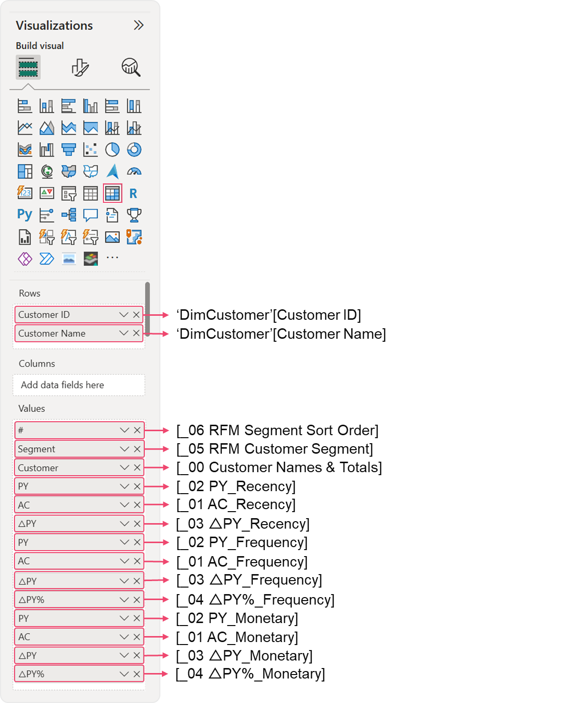 Setting up the table
Step 5.4: Cleaning Up the Labels and Adding Highlights
1. Renaming the Columns
To keep the report clean, we will simplify the column names. However, timing is everything. You must finish all your settings (like decimal places or colors) before you rename the columns.
-
AC: Your data for the current year.
-
PY: Your data from the previous year.
-
△PY: The total difference (increase or decrease) between years.
-
△PY%: The percentage change between years.
⚠️ Important: Configure each column’s settings first, then rename them. If you rename them to the same name (like "AC") before you are done, the system will force them to use the exact same settings.
2. Using Colors to Spot Problems (Conditional Formatting)
We use red text to highlight customers who might be leaving or who haven't bought anything new.
- Last Purchase (Recency): If a customer hasn't bought anything in 365 days or more, the number will turn red. This warns you that it has been a full year since their last visit.
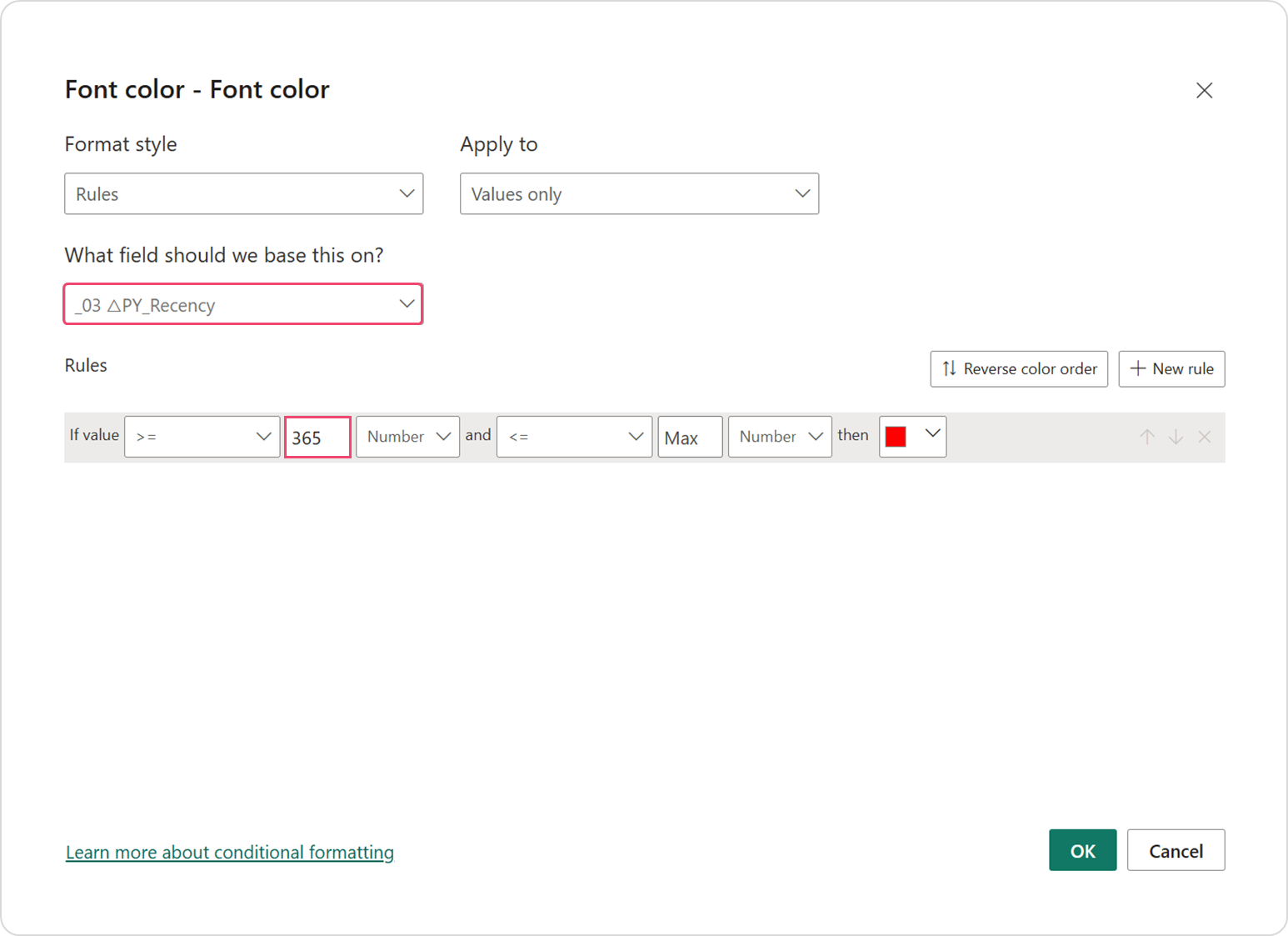 Highlighting the gap in days since the last purchase.
- Activity (Frequency & Money): If the difference between this year and last year is 0 (or 0%), the number will turn red. This shows the customer has stopped spending or visiting entirely.
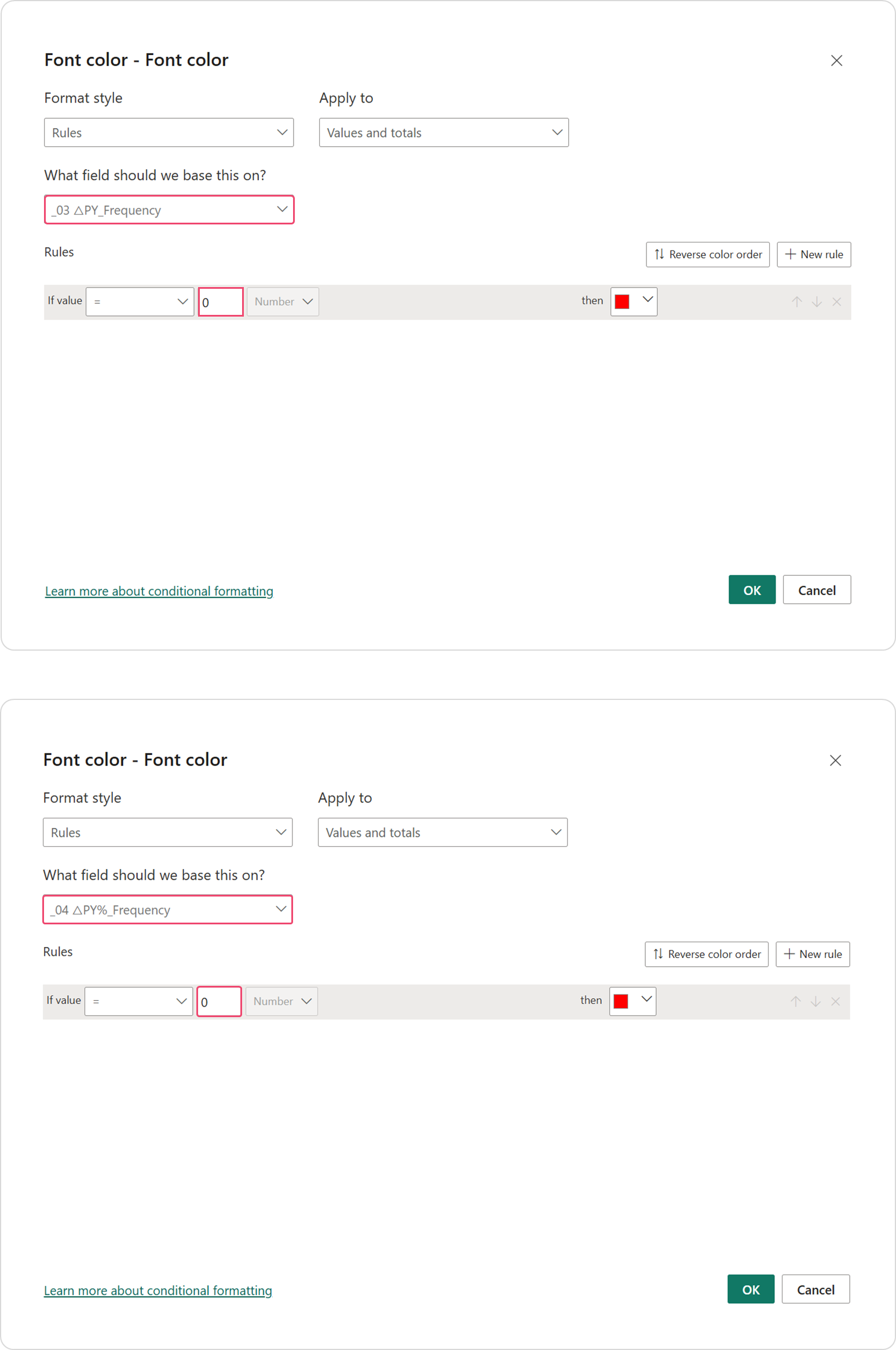 Highlighting the difference in total transaction counts
- Identifying Inactive and New Customers: To help you focus on active business, we use colors to separate different types of customers. If a customer’s spending hasn't changed at all (0% change), their information will turn grey to show they are inactive. On the other hand, brand new customers will be highlighted in blue. You can spot them easily because they show a 100% increase in spending compared to last year.
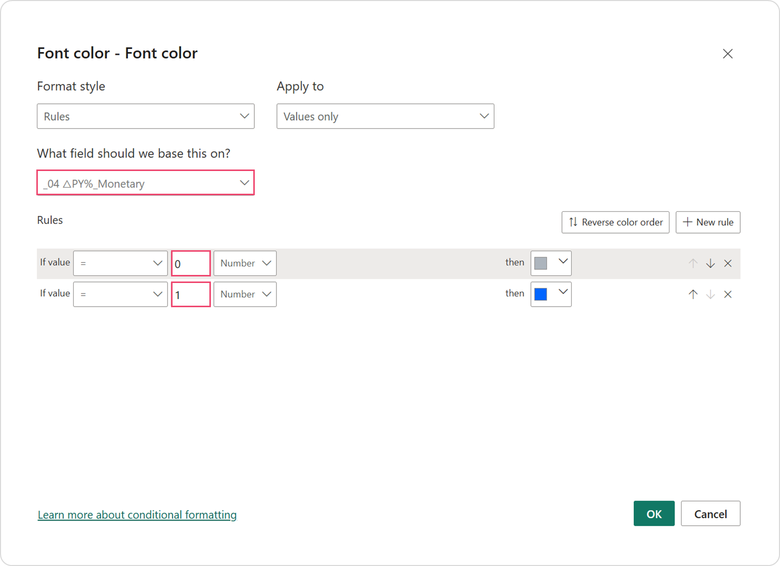 Highlighting the churned and new customers
Reference
Table template 01 • IBCS - International Business Communication Standards